Extreme Value Analysis Software for Weather and Climate

extRemes (version >= 2.0) and in2extRemes¹ are R packages for statistically analyzing extreme values of a data set. in2extRemes is a point-and-click software tool that operates many of the command-line functions from the extRemes (version >= 2.0) package.²

Sign up to receive updates when new package versions are submitted to CRAN (note that this list does not allow members or others to send emails to it, only the list administrators).

You may want to join the User Group for extRemes. The user group is intended for users to discuss issues about EVA and/or extRemes/in2extRemes with each other. Issues regarding bugs, etc., should still be sent to the maintainer (currently, Eric Gilleland).

CRAN landing pages for extRemes and in2extRemes.

---

¹These software packages were funded by the National Science Foundation (NSF) through the NCAR Weather and Climate Impact Assessment Science Initiative with additional support from the NCAR Geophysical Statistics Project (GSP).

² Originally, extRemes (versions < 2.0) was (primarily) point-and-click software running functions from the R package, ismev. The new package, in2extRemes, now takes on the point-and-click role, and extRemes has only command-line functions. The package ismev is still available on CRAN.

Extreme value analysis (EVA) is used primarily to quantify the stochastic behavior of a process at unusually large (or small) values. Particularly, such analyses usually req uire estimation of the probability of events that are more extreme than any previously observed. Many fields use EVA including: meteorology, hydrology, finance and ocean wave m odeling to name just a few.

Many statistical analyses concern sums or averages of random variables, and often rely upon limiting results such as the Central Limit Theorem to justify use of the normal ( or bell-shaped) distribution. When interest is in extremes, the bulk of the data may be misleading, and the normal distribution is not appropriate. A similar theorem to the Cen tral Limit Theorem, the Extremal Types Theorem, provides justification for using a family of distributions (in the univariate setting, similar results hold for multivariate ana lysis) known as the generalized extreme value (GEV) distribution. This, or analagous results for threshold excesses, are often the focus of EVA.

For more about EVA, see Rick Katz's page on extremes

• Installation
• Quick Start Guide
  
      extRemes
      in2extRemes

  Installation

  To install R, please visit The R Project for Statistical Computing for instructions. If you are intending to use the point-and-click software package in2extRemes, it relies on the Tcl/Tk tools, so be sure to install R with those tools (generally not the default!). They are not needed for extRemes version >= 2.0. Note also that for Mac users, the X Quartz package must be installed.

  Once R has been installed, open an R session. To install in2extRemes, type:
  
  install.packages("in2extRemes")

  The above command will install extRemes automatically, as well as other required packages. To install only extRemes, type:
  
  install.packages("extRemes")

  Installation need be done only once, but you can make sure you have the most recent version of your packages by typing update.packages() at any time (after installing them) from your R prompt.

  Once installed, the packages must be loaded into your R session (every time) in order to use them. To load in2extRemes, type:
  
  library(in2extRemes)

  The above command will automatically load extRemes and all other required packages. If you are only using extRemes, then load using library(extRemes).

  To begin using the in2extRemes window interface, type:
  
  in2extRemes()

  Quick Start Guide

  extRemes

  library(extRemes)
  data(Fort)
  names(Fort)
  
  bmFort <- blockmaxxer(Fort, blocks = Fort$year, which="Prec")
  names(bmFort)
  
  plot(Fort$year, Fort$Prec, xlab = "Year",
          ylab = "Precipitation (inches)",
          cex = 1.25, cex.lab = 1.25,
          col = "darkblue", bg = "lightblue", pch = 21)
  
  points(bmFort$year, bmFort$Prec, col="darkred", cex=1.5)
  
  # Fit a GEV distribution to annual maximum Precipitation
  # in Fort Collins, Colorado, U.S.A.
  fitGEV <- fevd(Prec, data = bmFort)
  fitGEV
  plot(fitGEV)
  plot(fitGEV, "trace")
  
  # Select a threshold for daily data from above.
  threshrange.plot(Fort$Prec, c(0.1, 2), type = "PP")
  
  # Fit the PP model to the daily data from above.
  fitPP <- fevd(Prec, data = Fort, threshold = 0.395,
          type = "PP", units = "inches")
  fitPP
  plot(fitPP)
  
  atdf(Fort$Prec, 0.395)
  
  extremalindex(Fort$Prec, 0.395, blocks=Fort$year)
  
  dcFort <- decluster(Fort$Prec, 0.395, r = 9)
  plot(dcFort)
  

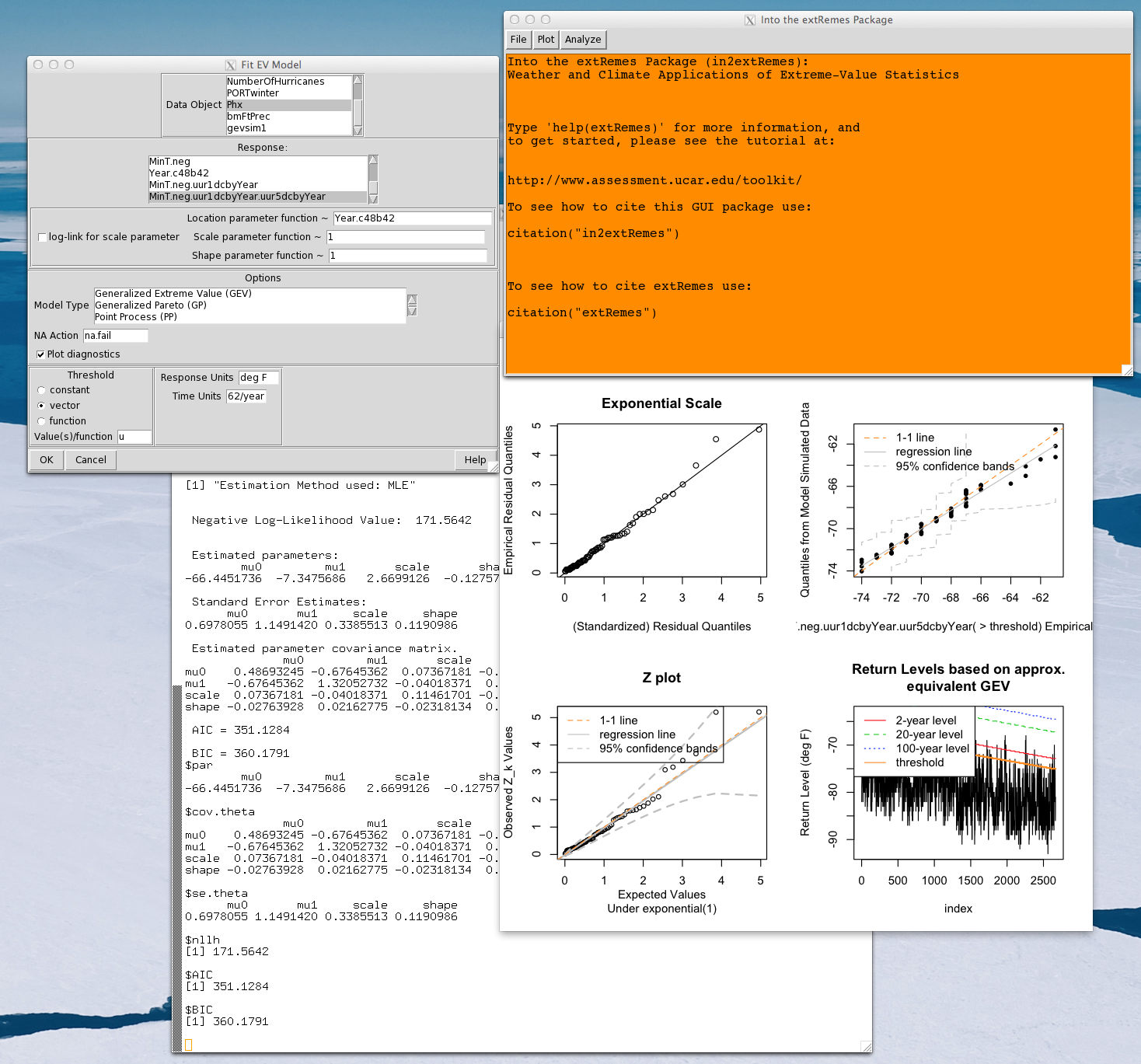
  in2extRemes

  library(in2extRemes)
  
  data(Fort)
  FortCollinsPrecip <- as.in2extRemesDataObject(Fort)
  
  # Open the main GUI dialog.
  in2extRemes()
  
  

  Select File > Block Maxima

  Select FortCollinsPrecip from Data Object

  Select Prec from Find block maxima of ...

  Select year from Blocks

  Type bmFtPrec in Save As (in R) field, and click OK.

  Fit the GEV to the annual maximum precipitation (inches) in Fort Collins, Colorado, U.S.A.

  Select Analyze > Extreme Value Distributions

  Select bmFtPrec from Data Object

  Select Prec from Response

  Select Generalized Extreme Value (GEV) from Model Type

  Check Plot diagnostics checkbox

  Type inches in Response Units field, and click OK

• extRemes >= 2.0
• in2extRemes

Short Courses

9th International Extreme Value Analysis Conference Satellite Workshop on Statistical Computing for Extremes, 14 June 2015, Ann Arbor, Michigan. (Univariate part: Presentation slides, pdf, Practice Problems, pdf)

Gilleland E. Short course: An introduction to the analysis of extreme values using R and extRemes. Graybill VIII/6th International Conference on Extreme Value Analysis. Colorado State University, Fort Collins, Colorado. 22-26 June 2009.

Gilleland E. Intense course for young researchers on R Statistical software for climate research with an introduction to extreme value analysis, Interdisciplinary Workshop: Effects of climate change: coastal systems, policy implications, and the role of statistics Workshop. 16-20 March 2009, Preluna Hotel and Spa, Sliema, Malta.

Katz RW, 2009: "Problem application: Exercise session on analyses of extremes." American Meteorological Society Short Course on Statistics of Extreme Events, Phoenix, AZ. (pdf lecture notes)

Katz RW, 2008: "Background on extreme value theory with emphasis on climate applications." Short Course on Statistics of Extremes in Climate Change, Michigan State University. (pdf lecture notes)

Katz RW, 2008: "Application of extreme value theory to climate change." Short Course on Statistics of Extremes in Climate Change, Michigan State University. (pdf lecture notes)

Citing R and R software packages

You can see how to cite the R programming language in a paper or presentation using the following command in your R session:

citation()

Similarly, to cite extRemes, use:

citation("extRemes")

And, to cite in2extRemes, use:

citation("in2extRemes")

Publications/Presentations about, or making use of, extRemes (all versions) and in2extremes

    About extRemes and in2extRemes
    Weather and Climate
    Other research areas

About extRemes (all versions) and in2extRemes.

Gilleland, E. and R. W. Katz, 2006: Analyzing seasonal to interannual extreme weather and climate variability with the extremes toolkit (extRemes), 18th Conference on Climate Variability and Change, 86th American Meteorological Society (AMS) Annual Meeting, 29 January - 2 February, 2006, Atlanta, Georgia. P2.15 (pdf).

Gilleland, E. and R.W. Katz, 2011: New Software to analyze how extremes change over time, Eos, 92 (2), 11 January 2011, 13 - 14.

Gilleland, E., M. Ribatet and A. G. Stephenson, 2013: A software review for extreme value analysis. Extremes, 16 (1), 103 - 119, DOI: 10.1007/s10687-012-0155-0 (available online at http://www.springerlink.com/openurl.asp?genre=article&id=doi:10.1007/s10687-012-0155-0).

Stephenson, A. G. and E. Gilleland, 2006: Software for the Analysis of Extreme Events: The Current State and Future Directions, Extremes 8, 87 - 109.

Weather and Climate Applications

Abeysirigunawardena, D. S., E. Gilleland, D. Bronaugh, 2009: Extreme wind regime responses to climate variability and change in the inner-south-coast of British Columbia Canada. Atmosphere-Ocean, 47, (1), 41 - 61.

Bodini, A. and Q. A. Cossu, 2008: Analysis of precipitation trends during 2nd half of the 20th century in an area of Sardinia (Italy) at high hydrogeological risk. CNR-IMATI Technical Report 08.11. Available at http://www.mi.imati.cnr.it/iami/papers/08-11.pdf

de Oliveira, M. M. F., N. F. F. Ebecken, J. L. F. de Oliveira and E. Gilleland, 2010: Generalized extreme wind speed distributions in South America over the Atlantic O cean region. Theor. Appl. Climatol., 104, (3 - 4), 377 - 385, doi:10.1007/s00704-010-0350-3.

Guttorp, P. and Xu J., 2010: Climate change, trends in extremes, and model assessment for a long temperature time series from Sweden. Environmetrics, 22, (3), 456 - 463, doi:10.1002/env.1099.

Heaton, M. J., M. Katzfuss, S. Ramachandar, K. Pedings, E. Gilleland, E. Mannshardt-Shamseldin, and R. L. Smith, 2010: Spatio-temporal models for large-scale indicators of extreme weather. Environmetrics, 22, 294 - 303, doi:10.1002/env.1050.

Helminen, J., A. Venäläinen and A. Vajda, 2005. The occurence of extreme precipitation values in Finland during summer (May-September). 4th Conference on Extreme Value Analysis: Probabilistic and Statistical Models and their Applications, 15 - 19 August, 2005, Gothenburg, Sweden (pdf).

Katz, R. W., G. S. Brush, and M. B. Parlange, 2004: Statistics of extremes: Modeling ecological disturbances. Ecology, 86, 1124 - 1134 (pdf).

Lu, J., 2007: Local effects of global warming. Masters Thesis, Dept. of Mathematics and Statistics, Texas Tech University, Clyde F. Martin, Committee Chair. Selected as Women's Studies Best Graduate Student Paper.

Mares, C., I. Mares, and A. Stanciu, 2009: Extreme value analysis in the Danube lower basin discharge time series in the twentieth century. Theor. Appl. Climatol., 95, 223 - 233, doi:10.1007/s00704-008-0001-0.

Pirazzoli, P. A. and A. Tomasin, 2007: Estimation of return periods for extreme sea levels: a simplified empirical correction of the joint probabilities method with examples from the French Atlantic coast and three ports in the southwest of the UK. Ocean Dynamics, 57, 91 - 107.

Pirazzoli, P. A., A. Tomasin, and A. Ullmann, 2006: Extreme sea levels in two northern Mediterranean areas. J. Mediterranean Geography, 108, 59 - 68. Available at: http://mediterranee.revues.org/170

Sanabria, L. A. and R. P. Cechet, 2007: A statistical model of severe winds. Geoscience Australia Record 2007/12. Available at: http://www.ga.gov.au/image_cache/GA10911.pdf

Schleip, C., D. P. Ankerst, A. B&oouml;ck, N. Estrella, and A. Menzel, 2012: Comprehensive methodological analysis of long-term changes in phenological extremes in Germany. Global Change Biology, 18, 2349 - 2364, doi:10.1111/j.1365-2486.2012.02701.x.

Unkašević, M. and I. Tošić, 2009: Changes in extreme daily winter and summer temperatures in Belgrade. Theor. Appl. Climatol., 95, 27 - 38, doi:10.1007/s00704-007-0364-7.

Venäläinen, A., K. Jylhä, T. Kilpeläinen, S. Saku, H. Tuomenvirta, A. Vajda, and K. Ruosteenoja, 2009: Recurrence of heavy precipitation, dry spells and deep snow cover in Finland based on observations. Boreal Environment Research, 14, 166 - 172.

Walter, M. D., 2008: Application of the Statistical Theory of Extreme Values to Heat Waves. Significant Opportunities in Atmospheric Research and Science (SOARS) Program. (pdf)

Wise, E. K., 2009: Climate-based sensitivity of air quality to climate change scenarios for the southwestern United States. Int. J. Climatol., 29, 87 - 97, doi:10.1002/joc.1713.

Wolters, D., 2007: A method to investigate the time evolution of the probability distribution of high temperature extremes in The Netherlands, applied to the extremes in the period of May 2006-April 2007. MSc study project, Wageningen University, supervisors: dr. Leo Kroon and drs. Paul Torfs. (pdf)

Other research areas

de Alba, E., J. Zúñiga, and M. A. Ramírez Corzo, 2008. Measurement and transfer of catastrophic risks: A simulation analysis. Institute of Insurance and Pension Research (IIPR) Report 2008-03.

Denny, M. W., 2008. Limits to running speed in dogs, horses and humans. J. Experim. Biol., 211, 3836 - 3849, doi:10.1242/jeb.024968.

Fujita, M., 2007. Separation and Airspace Safety Panel (SASP) meeting of the working group of the whole. Twelfth meeting of the International Civil Aviation Organization, Santiago, Chile, 5-16 November 2007 (pdf)

OBrien, E. J., A. Bordallo-Ruiz and B. Enright, 2014. Lifetime maximum load effects on short-span bridges subject to growing traffic volumes. Structural Safety, 50, 113 - 122, DOI: 10.1016/j.strusafe.2014.05.005

Saito, S., S. Aburatani, and K. Horimoto, 2008. Network evaluation from the consistency of the graph structure with the measured data. BMC Systems Biology, 2:84, 14 pp., doi:10.1186/1752-0509-2-84 (pdf)

Updates

Version 2.0-11 (available on CRAN soon): New (parametric) boostrap inference functionality has been added via xbooter and xtibber. Both of which are w rapper functions to booter from package distillery. The original parametric bootstrap remains (and will remain) available via the ci< /tt> function. A minimal amount of bivariate EVD fitting has been added in the form of fitting bivariate POT models to threshold excesses. The logistic and mixed beta dependence functions are available with bootstrap resampling for inference. See the help files for fbvpot and bvpotbooter.

Version 2.0-10: The dependency on the car package has been removed. The only noticeable change is that the qq-plot for the inter-excee dance times of PP model fit against the theoretical quantiles of the mean-one exponential distribution (the so-called Z-plot, as well as the W-plot) has c onfidence bands that are calculated differently (and will likely be wider). The bands are now calculated the same way as the qq2 option from the plot method. The dependence on the car package often made it difficult to install extRemes, and only the qqPlot function had previously been used from car.

Version 2.0-9: A user-found bug in the summary function to fevd under the Bayesian setting that caused the function to error out has been fixed.

Version 2.0-8: A bug in the MRL plot code was found by a user in the calculation of the confidence intervals, and this problem has been fixed. Another user-found bug involved the GMLE profile likelihood that did not utilize the penalty term for the GMLE, thereby giving erroneous values. This problem has also been fixed.

Some user suggestions have been incorporated, including: (i) fevd plot function now invisibly returns the values plotted provided the type argument is not "primary" (i.e., the default); (ii) the fevd plot function (and threshrange.plot) will now return the par arguments back to what they were before the function was called; (iii) a bug in the qq2 type of plot was found and fixed; and (iv) ellipses are now passed to the ci function in the threshrange.plot function so that other ci methods can be used.

The version also contains the new citation information for the package.

Version 2.0-7: A new heat wave magnitude index function (hwmid) has been added; as supplied by Simone Russo. It calculates the index described in the recently published paper: Russo, S., J. Sillmann, E. Fischer, 2015. Top ten European heatwaves since 1950 and their occurrence in the coming decades. Environmental Research Letters, 10, 124003, doi:10.1088/1748- 9326/10/12/124003.

Version 2.0-6: The print method for the ci function was printing incorrect information for the normal approximation of stationary models for the parameters when only one parameter's CI's are estimated. Additionally, the initial values to the profile likelihood function (profliker) were not generally optimal making it difficult to get good profile likelihoods (and subsequently CIs). These bugs have been fixed.

Version 2.0-5: A couple of users found two different bugs in fevd when using the GMLE method option (primarily for models with parameters that vary). Essentially, the old code should work fine for models whose parameters do not vary, though it was strictly incorrect. This version fixes that problem, and extends the Martins and Stedinger GMLE framework to that in, e.g., El Adlouni et al. (2007, WRR, 43: W03410, doi: 10.1029/2005WR004545). Also, a typo in the fevd help file concerning the time.units argument has been fixed. It used to say that it would take plural names, such as "minutes", when in fact, it wants them to be singular, e.g. "minute".

Version 2.0-4: The function pevd erroneously converted the scale parameter to that of the GP, then switched the type argument to "GEV" instead of "GP." Now, it no longer converts the scale parameter, but still switches the type argument to "GEV" in order to assume that that is what was intended by the user.

A function, written by Simone Russo, called hwmi is introduced, which calculates the "Heat Wave Magnitude Index."

A function called abba, written by Alec Stephenson, is introduced. It is an experimental function that implements the MCMC methodology for fitting spatial extreme value models as proposed in Stephenson et al. (2015, J. Appl. Meteorol. and Climatol., in press).

Version 2.0-3: Minor bug introduced from previous version fixed.

Version 2.0-2: A user-reported bug in qevd was found whereby the lower.tail argument was backwards for the POT models (it was correct for the BM models). This bug has been fixed. Additionally, another user-reported mis-communication from the fevd help file concerning the "GMLE" optimization method has been corrected.